The recent U.S. election was one of the most controversial and closest ever, and turnout percentage may be the highest in a century. Still, 37% of the voting age population did not vote. The traditional explanation for why people don’t vote is that they feel their vote won’t affect the outcome. Given the huge numbers involved in national elections, this is a rational calculation.
Even the famously close 2000 Presidential election was decided by 537 votes in Florida: a tiny percentage margin, but well beyond the reach of being changed by a few individual voters. State and local elections are a different matter. In a lifetime of elections in an electorate of 1000 people, with sentiment more or less equally split between two factions, an individual would be almost sure to encounter an election in which their vote could affect the outcome.
An equally-split electorate equates to a “random voting model” (votes cast randomly), a model that underlies much academic research into how much power voters have. Statistical and political science researchers have devoted a surprising amount of attention to defining and studying this issue. Andrew Gelman et al, in “The Mathematics and Statistics of Voting Power” (2002), defines voter power as “the probability that a single vote will be decisive.” Much of this research was propelled by a decline in voter turnout for U.S. presidential elections in the latter half of the 20th century.
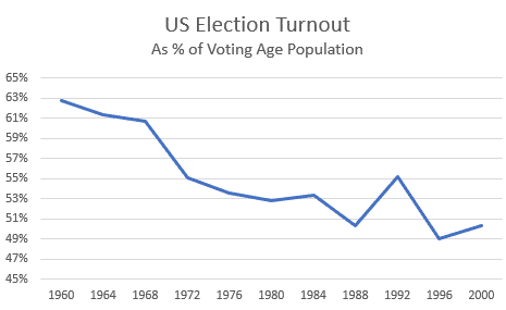
Figure 1: U.S. Voter Turnout
The Random Voting Model
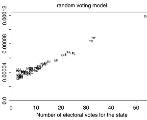
Research into voter power shares a common theme with much of the political and economic literature of the time: a fascination with mathematical manipulation not moored in reality. For example, one popular model was the “random voting model,” which assumed that votes were cast randomly and then explored implications for voter power under different voting systems. In the U.S. presidential electoral system, this led to an assessment that voter power was proportional to state size and electoral votes. The bigger your state, the more voter power you had. The probability of a tied election declines proportionally to the square root of population, while the weight of a vote increases proportionally to population itself. This is illustrated in Figure 2, where voter power, on the y-axis, incorporates a weight reflecting state population. The probability that an individual’s vote would be decisive is tiny (on the order of 1 in 20,000), but it is calculable.
Figure 2: Voting Power Under Random Voting Model
Of course, votes are not cast randomly; this assumption was made in order to produce a stochastic model to play with. The reality is that many states, including large ones like California and New York, typically have lopsided elections that depart far from the random voting model. Most political observers would agree that the U.S. electoral college system, in which each state starts with two votes, regardless of population, then gets additional votes depending on population, is biased in favor of voters who live in small states. Nonetheless, the random voting theory achieved such popularity that many researchers concluded that, because of the hypothesized close elections in big states based on random voting, the voters there had more influence than those in small states. Gelman et al cite work by Banzhaf (1968), Brams and Davis (1974),Mann and Shapley (1960), Owen (1975) and Rabinowitz and Macdonald (1986) all concluding, as Banzhaf did, that “citizens of the large states had an excessive amount of voting power.” Gelman et al, after incorporating actual election behavior (an injection of reality into social science research that was novel at the time), painted a picture in which state size did not appear to be associated with voter power.
Figure 3: Modeling Voter Power by Incorporating Empirical Variation from Random Voting
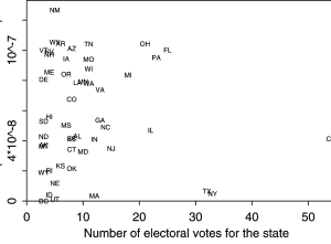
Random voting biases results towards a 50/50 outcome, which has the highest probability of producing a tie and, hence, maximizes individual voter power. Where electoral preferences depart far from a 50/50 split (think California and New York), individual voter power is effectively non-existent. It is interesting to note that Gelman et al quantified this imbalance, and that voter power (y-axis) varied by a factor of more than 20, depending on the state.
Rational Choice
Why people bother to vote emerged as a major preoccupation of political scientists who studied rational choice theory. This theory suggests that individuals have preferences and that, according to these preferences, different choice options have different utilities to those individuals. The utilities are derived from perceived costs and benefits of the options. People then make rational choices based on their assessments of the options open to them and the associated utilities. The conundrum of why people vote when an individual’s vote would seem to make no difference was a “major theoretical puzzle,” in the words of John Aldrich (Rational Choice and Turnout, 1994). For an individual, the act of voting, being virtually ineffectual, would seem to have no perceived benefit, but it would have a minor cost in time and effort.
Other researchers added game theory, in particular the minimax regret model. Consider a simple election, in which a voter is faced with the choice of voting for A, voting for B, or not voting. In each case, the regret caused by alternative outcomes is calculated, translated into utility, and the choice is made in such a way as to minimize the maximum regret that might result from a choice. This is really an exemplar of the general minimax strategy in which decision alternatives are arrayed according to the maximum loss from each alternative, and the alternative with the lowest maximum loss is chosen. Contrast this with the cautious optimist’s maximin strategy, to maximize the minimum gain, and the reckless optimist’s maximax strategy, to maximize the biggest possible gain. Finally, it is worth noting that both rational choice and game theory build on top of the voting power idea of having a decisive vote: they have at their foundation the possibility of a tied electorate, giving an individual a decisive vote.
The Decline of Rational Choice
The theory of rational choice declined as psychologists began publishing experiments illustrating that people are not fully rational. Rather than being highly logical thinking machines making decisions calculated to maximize their utility, humans form judgements quickly and impressionistically, often based on seemingly irrelevant issues. Alexander Todorov showed volunteers facial images for a fraction of a second and had them characterize the faces as to likeability and competence (and other characteristics). The images that the volunteers saw for a split second were actual candidates for political office.
70% of the time, the faces scoring high in competence, based on that split second viewing, were the winner of the actual election. Daniel Kahneman, in Thinking Fast and Slow, illustrates numerous experiments which decisions and judgements are often made on the basis of initial impressions, in ways that seem to contradict rational thinking. Another factor that diminished researcher interest into why people vote or don’t vote was the upswing in voting participation following the extremely close 2000 election.
Figure 4: Voter Turnout 1960 – 2020
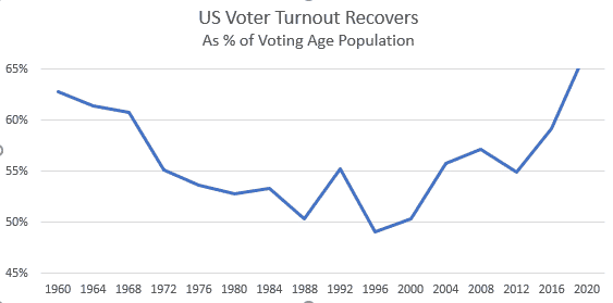
Declining voter turnout had been a worrying trend for political observers, worthy of study and explanation. With voter turnout increasing, the issue of why people vote persisted as a theoretical puzzle, but with diminished practical importance.
Close Elections
Extremely close elections, the predicate for the simplistic “random voting” theory, do happen, as evidenced by the recent results in Georgia (Biden leading by 0.3% a week after the election). But what about tied elections, the case where the political scientists get excited about their models? They are surprisingly common.
Wikipedia lists 15 tied elections over the past 50 years in the U.S. and Canada. Total vote counts ranged from 1500 to over 30,000, split equally between the candidates. Nearly all listed were for state or provincial legislative seats. Looking at the jurisdictions, several were repeaters: Massachusetts had three tied elections, Virginia two, and Quebec two. This frequency pattern suggests that the list is incomplete. The tied elections were decided by drawing lots, picking a sealed envelope from a cup, drawing a name from a hat, the vote of the presiding officer, or the vote of the legislative body in contention. In 1891, a tied election in Indiana was settled by a footrace between the candidates.