Five years ago last month, the psychology journal Basic and Applied Social Psychology instigated a major debate in statistical circles when it said it would remove p-value citations from papers it published. A year later, the American Statistical Association (ASA) released a statement on p-values that responded to growing concerns that the traditional p-value was not an appropriate gatekeeper to publication of scientific studies. Also needed are “good study design, … understanding of the phenomenon under study, interpretation of results in context, complete reporting and proper logical and quantitative understanding of what data summaries mean.” As Ron Wasserstein, the ASA’s Executive Director, put it “The p-value was never intended to be a substitute for scientific reasoning.”
The genesis of this statement was criticism in the research community that many low quality (and often meaningless) studies were being published simply because investigators had rooted around in data long enough to find a significant p-value when comparing variable x to variable y.
Origins
The first example of the logic behind p-values is a publication by John Arbuthnot, the Scottish satirist and mathematician. Arbuthnot reviewed records of births in London from 1629 to 1710, and found that in every year the number of males exceeded the number of females. If the probability of a birth being a boy or a girl is the same, 50/50, then the chance of 82 years in a row yielding more boys than girls was infinitesimally small. Arbuthnot concluded that, since chance was not responsible, God must be. This is the logic of a hypothesis test, with the null model being “chance is responsible,” and the alternative hypothesis being “God must be responsible.” You can see that Arbuthnot’s alternative falls short by today’s standards – the null and alternative hypotheses do not exhaust all possibilities.
It was not until R.A. Fisher’s work with agricultural experiments in the 1920’s, though, that hypothesis testing became an important part of the statistician’s work. His “Lady Tasting Tea” example, published in his 1935 book The Design of Experiments, clearly set forth the logic.
The Lady Tasting Tea
In Fisher’s scenario, loosely based on reality, an acquaintance of his claimed to be able to determine, when tasting tea, whether the tea was poured into the cup first, or the milk. Fisher prepared 8 cups for her, 4 with the tea poured first and 4 with the milk poured first. The cups are presented in random order. The null hypothesis is that the lady has no ability to tell one group from the other. In the event, the lady was able to guess all 8 cups correctly. Under the null hypothesis, this would have been by chance. What is the chance of guessing all 8 cups correctly?
There are 70 different ways the cups could be ordered, so the probability of guessing the correct ordering, just by chance, with no real ability to discern, would be 1 out of 70, or 1.36%. We could also arrive at this probability by repeatedly shuffling four 1’s and four 0’s, and seeing how often we match a single particular “winning” permutation. Fisher judged 1.35% too small to be attributable to chance and concluded the lady’s correct guess was due to real tea tasting ability. The term “null hypothesis” came from Fisher, as something to be rejected in favor of the alternative, which is what really interests us:
“We may speak of this hypothesis as the ‘null hypothesis’ […] the null hypothesis is never proved or established, but is possibly disproved, in the course of experimentation.”
Fisher was also responsible for the standard of 5% significance, as a threshold level for being judged too extreme to be attributable to chance. Fisher did not attempt any rigorous justification for the 5% level, merely saying that it seemed convenient and reasonable. You can read more in Fisher and the 5% Level by Steven Stigler.
Fast Forward to Today – Hypothesis Testing at Volume
In those early days, the need to avoid being fooled by chance was taken for granted, and, over time, hypothesis testing with a 5% level of significance got built into the statistical machinery. Drug regulators and journal editors began to demand proof of statistical significance before accepting studies. However, there is little in the literature to point to widespread cases where researchers were, in fact, being fooled. Now, there is.
There are two main areas where “hypothesis testing at volume” offers opportunities to be fooled by chance. Unfortunately, the traditional p-value offers a remedy to neither.
Academic Research
Academic research by scholars seeking publication. Not only is the sheer volume of this research overwhelming (one source puts the number of papers published annually at 2.5 million), but any given study may be the tip of an iceberg that embodies a large number of questions and comparisons, with only the iceberg’s tip achieving publication (because it tested “significant”). There simply aren’t that many interesting findings awaiting discovery out there every year, hence the “reproducibility crisis” in research — many published studies turn out to fail when other scholars attempt to reproduce them.
The test of statistical significance was supposed to act as a filter to allow only truly meaningful studies to find the light of day, but the reverse has happened. Finding the magical and elusive 5% p-value became the only criterion for publication, causing other aspects of study design and interpretation, not to mention honesty in describing the full search through the data, to fall by the way. It is this phenomenon that forced the American Statistical Association to grapple with the issue of p-values as a filter to publication, resulting in the statement cited above.
There’s no evidence of large-scale abandonment of the p-value in research, though its reputation is definitely tarnished and the fracas may have caused editors to look more closely at papers submitted for publication from a broader statistical perspective than simply the p-value.
Genetic Research
Knowledge of human genetics is advancing by leaps and bounds, and so is the quantity of data. Of paramount interest is the association between genetic characteristics and disease. Microarray DNA analysis provided data on the actions of thousands of genes at once, so naturally researchers are keen to learn whether, for a specific disease, there is a connection with the particular expression of a gene (i.e. whether that gene differs significantly between people who have the disease and those who don’t).
Large Scale Testing
Doing this type of research requires conducting thousands, perhaps millions of hypothesis tests (genes can have over a million DNA bases). Clearly the traditional alpha = 0.05 is an inadequate standard — running just 100 hypothesis tests at the 0.05 significance level will yield 5 “significant” results, even if there are no truly significant cases. A classical adjustment for this is the Bonferroni bound, which lowers the threshold for significance, i.e. makes it more difficult to declare a result significant. The Bonferroni bound simply divides alpha by the number of comparisons, and sets that as the bound for each test. This adjustment aims to control the overall probability of making a single false rejection (declaring a case significant when it is not) at 0.05.
This is a conservative bound when applied to the original small-scale research context of Bonferroni corrections, where N, the number of comparisons would typically be less than 20. In large scale testing, with N in the thousands or more, Bonferroni is considered too conservative.
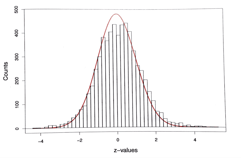
Efron and Hastie (in Computer Age Statistical Inference) describe a prostate cancer study of 102 subjects, split into 52 cancer patients and 50 normal controls. 6033 genes were studied to determine whether they differed significantly between control and cancer groups. Efron and Hastie plotted (in red below) the normal density curve that would represent the results of 6033 hypothesis tests if all cases were null. It is superimposed over a histogram of the actual results in the cancer study.
This issue is discussed in greater depth in chapter 15 of Efron/Hastie – you can download the PDF here, but the book itself is a grand tour of the discipline of statistics and well worth having in hard cover.
 [cancer curve]
The histogram matches the curve nicely, but you can see that actual results are bunched more at the tails and less at the top, suggesting that some hypothesis tests yielded truly significant results. Still, the Bonferroni adjustment for this study allowed only four hypotheses to be rejected, out of the 6033 tested.
False Discovery Rate
A more recent, and more popular approach in genetic testing is to control the rate of false discovery, q, instead of controlling the probability of a single false discovery. A typical choice is q = 0.10, meaning that you expect 90% of null hypothesis rejections to be correct – i.e. identifying real effects. 10% are allowed to falsely reject a null hypothesis. This is operationalized as follows:
- Rank order the hypothesis tests by p-value, smallest to largest, assigning each an index value i
- The decision threshold for each hypothesis test is (q/N)i — the i-th hypothesis test is rejected, and the effect declared“real,” if its p-value falls above that level.
This departs from the traditional strict concept of Type-1 error, but is more practical for large-scale testing. When applied to the cancer study, Efron and Hastie found that it allowed for 28 “findings” or rejected hypotheses, compared to the 4 allowed by Bonferroni.
Conclusion
As noted in the related short piece on false discovery in mental health research (The Depression Gene), many researchers lack a solid understanding of the statistical methods to control false discovery. Even the methods themselves are not settled – Efron and Hastie raise several important methodological questions, not the least of which is the somewhat arbitrary choice of q. So we can safely predict many more false discoveries.