False positives generated by detection systems are a huge problem. In the U.S., fire departments receive over 2 million false alarms per year. They put personnel at risk, cost millions of dollars, and may hinder a response to a real fire. False alarms from smoke detectors cause many people to simply disable them. If network intrusion detection systems frequently signal “intrusion” when nothing’s wrong, system administrators begin to ignore them. The key decision factor is the estimated probability that the alarm is real. If it’s 95%, you pay attention; the system is worthwhile. If it’s 5%, the system is more of an annoyance (and possibly worse).
To the lay person, this key probability would be expressed as the “false positive rate,” meaning the proportion of FP’s among all positive test/detection results. “Suppose a screening test has a 40% false positive rate. If you get a positive result on your test, there’s a 40% probability it’s a false positive.”
But this is not what the false positive rate means in statistics. Rather, the false positive rate is the proportion of true negatives that are misclassified as positives. The idea is the same whether the detection system is a diagnostic medical test, a fire alarm, or a statistical or machine learning model. The idea is the same: a device to distinguish between classes.
About nomenclature: In statistics and machine learning, the class of interest, the more rare class, (typically designated as a “1,” while the other class is labeled as “0”) might be a fraudulent tax return, a defaulting loan, a web visitor who goes on to purchase. In medicine, the “1” is the disease or condition for which the person is being tested. In the firehouse, the “1” is notice of an actual fire, as opposed to a false alarm.
The denominator
False positive rate confusion is all about the denominator. The numerator is always false positives (0’s classified as 1’s). Common sense would have a denominator of “all records classified as 1’s.” In statistics, though, the denominator is “all true 0’s.”
“False positive rate” is the label on the x-axis in many Receiver Operating Characteristics (ROC) charts (see this blog for more on that subject). Intrinsically, though, it is not a natural or useful metric. When you look only at the actual 0’s, you are interested in knowing how well the detection system classifies them, so your numerator would probably be “true 0’s.” The natural metric would be “proportion of 0’s correctly classified,” termed precision (in data science) or, equally, specificity (in medicine).
When discussing false positives in a domain setting (finance, marketing, intrusion detection, medicine), it is probably better to use the term “false alarm rate,” if you mean the proportion of positive classifications that are erroneous. It comes closer to the practical importance of the idea, and has less presence in the formal definitions of statistics that might cause confusion.
False Discovery
You may also have encountered the related term “false discovery.” A false discovery is like a false positive, specifically in the context of hypothesis testing. A false discovery occurs when a hypothesis test incorrectly signals “significant.” In other words, a type 1 error. The term false discovery came into common use with the advent of large-scale hypothesis testing, especially in genetic analysis. Analysts investigate the action of thousands of genes at once, to explore whether a specific gene or set of genes might be responsible for a disease. In such a case, it is easy to be fooled by chance associations. If you perform 6000 hypothesis tests at the 5% significance level then, under the null model, you will expect 300 (5%) to falsely show “significant.”
This is the extreme case of the “multiple testing problem” in statistics. The standard statistical toolbox has devices such as the Bonferroni correction to adjust the p-value in the various tests so that the probability of being fooled in this way is controlled. The most stringent application of adjustments like Bonferroni will maintain the probability of making even one false “significant” finding at the desired level of 5%, for example by dividing alpha (the specified significance level) into equal portions for each test. If you’re conducting 3 hypothesis tests, then each hypothesis test has its significance threshold (alpha) reduced to 0.05/3 = .0167.

Carlo Emilio Bonferroni, Italian probabilist (1892 – 1960)
The classic adjustments like Bonferroni, though, were meant for relatively small numbers of hypothesis tests, not thousands of simultaneous ones. Generic researchers were frustrated at the classic criteria since it set such a high bar for statistical significance. If you’re doing hypothesis tests on 6000 genes, which is not uncommon, then each test must meet a p-value bar of .05/6000 = 0.000008.
Controlling The False Discovery Rate (FDR)
In genetic testing, the classical procedures have been largely replaced by rules to control the false discovery rate – the rate at which null hypothesis rejections turn out to be false rejections. So we shift from the highly conservative approach of controlling the probability of even one false discovery to the more relaxed approach of controlling the rate of false discoveries – FDR.
The formula for FDR is simple:
FDR = a/R where
a = falsely rejected hypotheses
R = all rejected hypotheses
FDR Control Rule
The formula is also not that useful, since we don’t know which rejections are false and which are true. More useful is a decision rule that can control the expected (but unknown) FDR at a specified level, commonly called q. In this decision rule, we rank all the p-values for the N tested hypotheses, from most to least significant, and accept them as significant up to the ith p-value, pi, which is the largest one for which
pi <= (i/N)q
The figure below depicts this graphically with hypothesis testing for genes that might be associated with prostate cancer. The rank of the p-values is shown on the x-axis, the p-value corresponding to a given rank is shown on the y-axis. The FDR control line is a line sloping up from the origin. As you move from left to right, considering the hypothesis tests in declining significance, hypotheses are accepted as significant, provided they fall below the FDR control line.
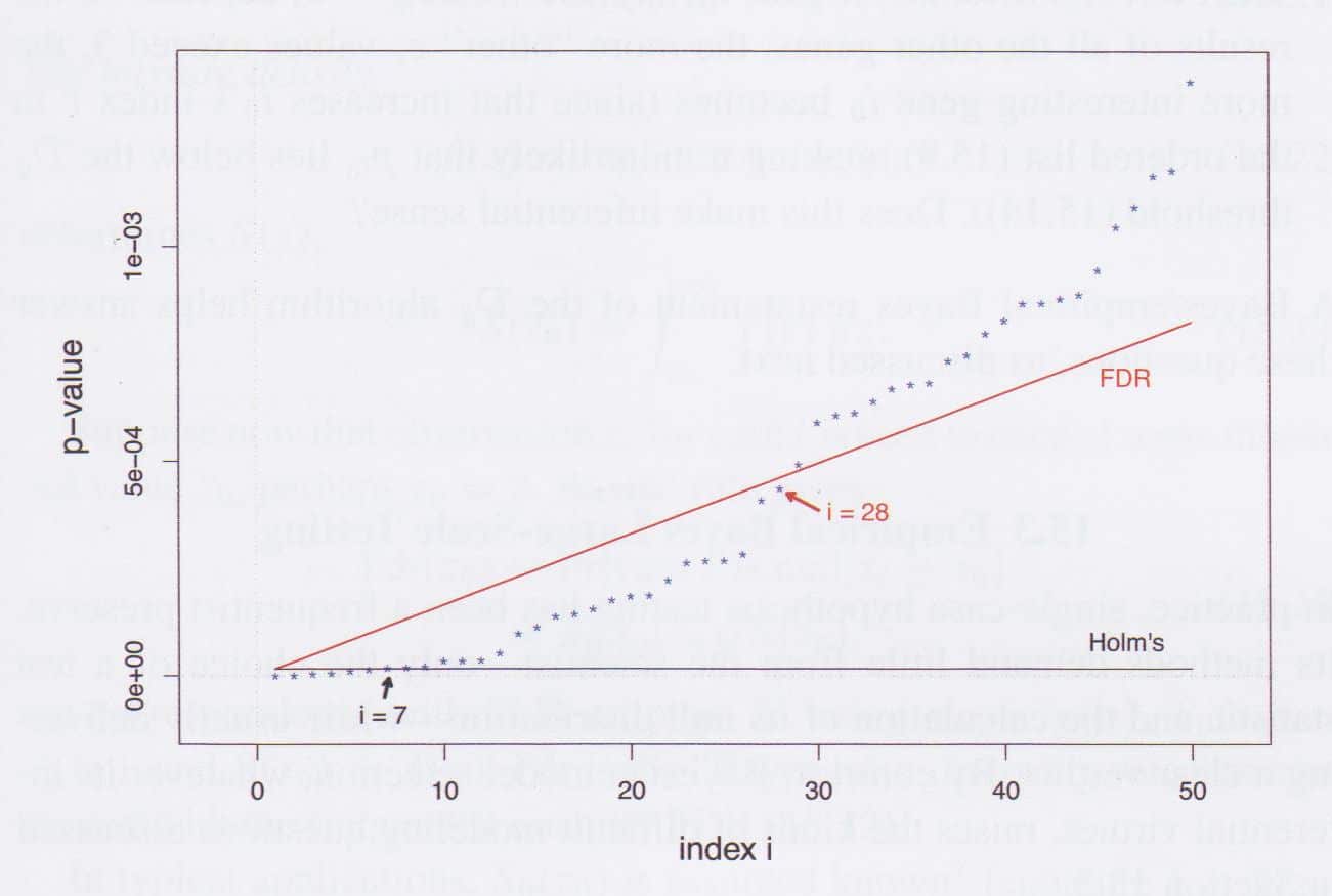
Figure: From Efron and Hastie, Computer Age Statistical Inference, fig. 15.3.
It is easy to see how this approach became popular among researchers: it allows far more results to meet the threshold for publication. A popular allowable rate for false discoveries, typically called q, is 10%.
Note that this q of 10% is not comparable to the traditional alpha of 5%. The latter is the probability of falsely rejecting a hypothesis under the null model, or, when divided up in a multiple testing setting, the probability of falsely rejecting one of the hypotheses. The former, q, is the rate at which rejected hypotheses are permitted to be falsely rejected.
You can see that, under the FDR criterion, 28 hypotheses have been rejected, i.e. 28 genes have been declared as likely connected to prostate cancer. Under a slightly more liberal version of Bonferroni ( “Holm’s criterion”), only 7 genes would be identified as significant.
Conclusion
The FDR approach to hypothesis testing, while popular among genetic researchers, has drawn criticism from statisticians. They wonder how q is selected, and worry that the selection might be arbitrary, and helps to lower the bar to publishing results. They also note that the research process is still embedded in the framework of statistical inference, and worry that the “rate of false discovery” as an idea does not square well with established standards of inference.