As the popularity of data science has grown, so too has advice on how to get jobs in data science. A common form of advice is a list of sample questions you might be asked at your job interview (see here and here for examples). Often, the list starts out with statistics, but beware: it may give bad advice.
Statistics is one of the key “legs” on the data science stool, but it also carries with it a century and a quarter worth of conceptual and mathematical scaffolding built in pre-computer times for non-big-data purposes. How do you sort out what’s important for data scientists? Here’s a guide for some often-cited topics.
Normal Distribution
There’s no question the normal distribution is popular in statistics, but it is less common in actual data than often supposed. One author’s list of 8 common data sources said to be normally-distributed had three items that were actually good examples of non-normal asymmetric distributions. For example, one item on the list, commuting time, is long-tailed right. (The average American commute is 27 minutes each way; there are many commuters with commute times well over an hour, but none with commute times less than zero.) By contrast, the normal distribution is valid and useful in describing most distributions of estimation errors (not the actual data values); errors are often normally-distributed even when the underlying data are not. This allowed the development of the probability distribution theory that undergirds early statistical inference (confidence intervals and hypothesis testing).
In the age of computer-based inference and resampling, this mathematical theory is less central. In fact, assuming normal distributions when not warranted can be hazardous. Assigning normal, rather than long-tail right, distributions to the returns of complex financial instruments was a contributing factor to the financial crash of 2008; that caused the probability of extreme events (“black swans”) to be underestimated.
Logistic and Linear Regression
While linear and logistic regression date back two centuries and a half-century, respectively, they remain popular in data science, despite the advent of increasingly powerful machine learning methods. They are fast, provide interpretable coefficients, protect better against overfitting, and give quick indications of feature importance. All of these characteristics make them particularly suitable for early-stage prototyping. They are by no means limited to the pilot phase, however. Google’s ad display algorithm, where speed is of the essence, employs logistic regression, according to a recent description.
Regression Metrics and Diagnostics
One downside of linear and logistic regression is software whose automatic regression output consists of numerous, mostly arcane, metrics. R-squared, adjusted R-sq, deviance, Cook’s distance, multiple tests for normality, p-values, AIC, the Wald test, the Hosmer Lemeshow test, and more. Most of these concern how well the regression model describes the data that it was trained on, and are calculated from that data. In data science, however, we are more interested in how well the model predicts new data, and we typically have holdout data available to assess a model’s performance. With linear regression, we use root-mean-squared-error, RMSE, which reflects the magnitude of a typical prediction error. With logistic regression, we use accuracy, or one of the other metrics used to measure classifier performance (lift, AUC, sensitivity, specificity, etc.) .
That said, data science does have a place for regression diagnostics, particularly the study of residuals, or errors in linear regression. Zillow’s home price estimating model (the “zestimate”) was refined early on by the use of regression diagnostics (it is now the subject of a Kaggle contest seeking further error reduction). Patterns in residuals offer an opportunity to improve predictive models. A cluster of higher residuals for a particular range of a specific predictor may indicate that some additional predictor or interaction may have been neglected by the model. As models age, examination of residuals is a useful item to include in the model review checklist.
Normality Assumptions
Talking of residuals, you will often encounter a list of assumptions that supposedly must be satisfied for a linear regression model to be valid. These assumptions concern the residuals: they should be independent of one another and normally-distributed, they should have a mean of zero and constant variance across different predictor ranges. As a data scientist, do you need to worry about this?
For the immediate purpose of deriving a predictive model, the answer is largely no. If a model does a good job of predicting out-of-sample data, end of story. For longer-range purposes, the answer becomes more of a “yes.” Violation of the assumptions does not mean a model is useless, rather it offers opportunities, as noted above, for the model to be improved.
P-Values
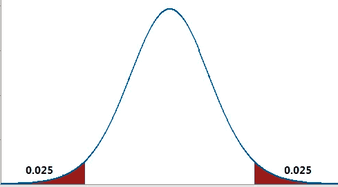
P-values are one of the most vexing aspects of statistics. They bedevil students, and many practitioners of statistics do not understand their original rationale and meaning, although they can report their values and use them. The p-value’s original reason-for-being was to keep you from being fooled by random chance variation into thinking that the unusual “pattern” you see in some data is meaningful. The human brain is very effective at reading meaning into random events, hence the need for this protection.
Some protection is afforded by the actual meaning of a p-value, applied to an event you perceive as interesting or unusual: “Assuming business as usual, i.e. there is no unusual pattern happening, how likely is it that the random flow of events could produce an occurrence as unusual as what you saw?” Unfortunately, after the gyrations required to operationalize this metric formally in decisions (null hypothesis, alternative hypothesis, significance level, rejection region, one-way versus two-way), most people have lost sight of its actual meaning.
Two-way p-value
Functionally, it has the greatest impact in academia, where a low p-value operates as a magic “green light” that allows you to get published. It is also important in medicine, where studies of new therapies must achieve statistical significance, as demonstrated by a low p-value. Its importance, though, has diminished in recent years as the awareness has spread of “p-hacking,” or the process of searching through lots of data and asking lots of questions until you find a relationship that is “statistically significant.”
There is not much of value for data scientists in the formal probabilistic interpretation of p-values, but they can be useful in the rapid piloting phase of model-building. For example, in feature selection, features with very low p-values can be marked for retention as useful predictors, while those with very high p-values can be eliminated. This process can be automated . In this context, p-values constitute more of an arbitrary score for ranking purposes than an accurate calculation of probabilities. And data science suggests a useful remedy for p-hacking: permutation of the target variable in a model (target shuffling) offers a flexible and intuitive tool for assessing whether relationships are real, or the product of random chance.
Central Limit Theorem
The Central Limit Theorem is a favorite of statistics quiz-makers. Basically, it says that even if the data behind an estimate (e.g. the mean) are not normally-distributed, the estimates calculated from different samples will be. This allows the use of formulas based on normal theory, for, say, calculating p-values. The Theorem’s applicability is not unlimited, it is invalidated if the departure from normality is too extreme. Teachers like the Central Limit Theorem because it produces nice simulations and plots that clearly show how larger sample sizes yield narrower distributions of a statistic like the mean. These visuals are a much more effective demonstration than mere words.
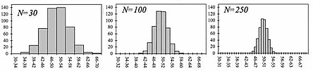
Distribution of the mean narrows as sample size (N) increases
Aside from nifty illustrations of the effect of sample size, the role of the Central Limit Theorem in data science, and even statistics nowadays, is not so central anymore. With the use of resampling and bootstrapping, it is not so important to have normally-distributed sample statistics.
Beyond the Minutiae
With excessive focus on formula-like details, key takeaways from statistics are often lost. We mentioned the natural human propensity to find patterns where none exist. Hypothesis-testing and p-values arose to counteract this propensity, but, unfortunately, the effort to understand them gets you so down in the weeds that you lose sight of the basic lesson: beware of finding patterns that aren’t really there.
Related to this is an intuitive understanding of variability and uncertainty: the appreciation of the role that random or unexplained forces play in life. Much of the machinery of statistics is constructed to quantify this, but it is possible to master the machinery without translating the underlying concepts to the decisions you encounter in life and business.
Two concepts from statistics do extend nicely into business and life in general without getting bogged down in technical mumbo-jumbo:
Regression to the Mean
The concept of regression to the mean was popularized in the 19th century by the statistician William Galton, who observed that tall men tended to have shorter sons. He termed it “regression towards mediocrity.” The idea is that if you see a data point or a set of data that are extreme, additional observations or sample from the same source are likely to be less extreme. A good example is the “rookie of the year” phenomenon. A rookie sports figure who does better than all the other rookies in a season has likely benefited from some degree of really good luck, luck that will probably be absent in the second year. Deprived of this extremely positive random element, his performance will decline in subsequent years and settle more towards his true long term capability.
Selection Bias
The rookie of the year is also an example of one type of selection bias – selecting an event or phenomenon specifically because it is interesting or extreme in some way. Selection bias, at its most general, refers to the selection of individuals for study in a systematically unrepresentative way. The more interesting cases of selection bias occur when the study group is selected for some non-random reason, and we jump to conclusions based on the characteristics of that group. A classic example is to look at successful businesses, and draw “lessons” about what a business should do to be successful. James Collins, in his 2001 best-selling book From Good to Great: Why Some Companies Make the Leap and Others Don’t, stepped into this classic selection bias trap. First he identified a dozen highly successful companies, then he described their common characteristics, then he concluded that these characteristics were what propelled them from mediocrity to “long-term superiority.”
The problem? When you select a subgroup, the members are bound to share some “feature values,” in the language of data science, just by chance. It is only human to associate these feature values with the basis on which you selected the group. A decade and a half after his book was published, Collins’ “long-term greats” turned out to be strikingly average. Half under-performed the Dow, one was bankrupt, one was bailed out by the government, and one was fined $3 billion after a scandal in which sales associates created fake bank accounts.
Conclusion
With a century and a quarter of development behind it, the field of statistics has accumulated a rich toolkit for data science, all at the disposal of the data scientist. We’ve pointed out some useful tools and some not-so-useful ones. A candidate for “best tool” is the statistical habit of thinking not in terms of measurements from definitive data, but rather in terms of distributions of estimates from samples that incorporate inherent error. Resampling, cross-validation and shuffling are all ways to generate additional samples and, from them, distributions of metrics.