Myth 1:  It’s All About Prediction

“Who cares whether we understand the model – as long as it predicts well!” This was one of the seeming benefits of the era of big data and predictive modeling, and it set data science apart from traditional statistics.  

Eric Siegel, in his popular book Predictive Analytics, termed it the prediction effect.  Siegel noted that, for predictive analytics to retain its magical halo, predictions do not have to be perfectly accurate, or even close to perfectly accurate, they just have to be consistently good.

But even Amazon, a company built on harnessing data to predict what you’ll want to buy, how to source it and where to stock it for fast delivery, discovered some limits of prediction when it developed an AI product to predict whether a job applicant would be a good fit with the company.  The black box text mining model was trained on current engineers’ assessments of an initial set of resumes.  It turned out that the black box model, when it read a resume, was essentially trying to find out whether the candidate was a man or a woman.  Regardless of what the engineers were thinking as they reviewed the resumes in the training set, they produced a set of labels for which it turned out that the best predictor of “good fit” or “bad fit” was the applicant’s gender.  Once the model figured that out, its job was done.

Obviously, pure prediction was not sufficient in this case.  Amazon needed to understand how the model was making its predictions and that applicant gender (not a permissible factor) was the key determinant.  The company finally came to the realization that more accurate predictions were not valuable: the problem lay in the engineers’ original judgments. Predicting those judgments more precisely would not solve anything.  In other cases, lack of full understanding of a model can lead to major implementation errors.  One common failure mode is “leaks from the future:” training a model on data that won’t be available at time of deployment.  In building a fraud model, for example, Elder Research had, at an early stage, a model with almost perfect predictive power.  Realizing this was too good to be true, they dug and found that “opened fraud investigation” was one of the training variables.  This variable in the training data benefited from significant investigative work suggesting a high fraud probability.  However, this information would not be available to a deployed model at the time of prediction.  Understanding and interpreting models’ decisions is now making a comeback, as the ethical and performance challenges of black-box models are becoming more apparent.

Old-fashioned linear models come equipped with all sorts of tools to facilitate diagnostics.  It’s easy to understand why a newly-minted data scientist might want to leave behind the complex and arcane baggage of statistical modeling, reflected in the litany of metrics that can be produced by a linear model (R-squared, adjusted R-squared, AIC, BIC, F-test, various sums of squares, p-values, etc.).  True, much of that is outmoded overkill, coming from the days when biometricians, psychologists, sociologists and other researchers were studying a given limited set of data and trying to explain it.  The better the model fit the data, the more explanatory power it was deemed to have.  The concept of overfitting was not well understood, since researchers typically used all the data to fit a model and could not observe the model’s performance with out-of-sample data.

Still, data scientists do a better job if they go beyond “fit and deploy.”  The diagnosis of residuals, for example, can tell you whether something important has been left out of the model, something whose inclusion might improve performance. Variable selection can produce a more parsimonious model, more robust against noise. Understanding how various predictors contribute to outcomes can facilitate a discussion with domain experts, which can often yield better models (e.g. through gathering more data, or including interaction effects).  There is much worthwhile in the techniques of traditional statistical modeling (as covered in the Social Science Statistics certificate program at Statistics.com) that is useful in the process of predictive modeling. 

Myth 2: Big Data are Better Data

Big data have transformed statistics and analytics, but have they made sampling and statistical inference obsolete?  This is the contention of Mayer-Schonberger and Cukier in their popular book Big Data: 

“The concept of sampling no longer makes much sense when we can harness large amounts of data. … a shift is taking place from collecting some data to gathering as much as possible, and, if feasible, getting everything: n=all.”

It is true that the era of big data has opened all sorts of doors by providing data scientists with useful treasure troves of data that were collected for other purposes.  Still, collecting truly “all” the data can be difficult and even impossible.  Getting all the data is often a far cry from tapping into existing observational data. The conveniently accessible data may differ in meaningful respects from the entirety, and data gathering efforts may be better spent on collecting a representative sample.  Consider the census, which used to be a door-to-door undertaking.

Capturing 80% or even 90% of the population is now relatively easy, done mostly by mail.  But what about transient or homeless populations?  People who split their time between Florida retirement homes and their permanent homes up north? Adult children who live part of the time at a school, and part of the time at home?  These groups may differ significantly from the rest of the population.  Getting that last 10%-20% to respond, and coding them correctly, is hard; it is not an easy proposition to get everything.

Census statisticians are not fans of the full census.  Instead of spreading their time and money on trying to find everybody, they would rather focus their efforts on reaching and verifying a smaller but statistically representative sample.  Criteria for a representative sample can be set beforehand, and money can be spent on repeated callbacks to get closer to 100% response.

Taking only the data that can be conveniently obtained can lead to bias – the hard to obtain data may differ systematically from the rest.  Another important factor is data cleanliness.  It is rare that “naturally occurring” data are ready for analysis.  They often require cleaning and preparation, which, in turn, may require the involvement of someone familiar with the data. This is much less costly with a sample of data, particularly in the prototyping phase.  Moreover, good models and estimates typically require only several thousand records.  If they are properly sampled and provide sufficient data on key predictors, there will be minimal improvement from adding hundreds of thousands or millions more.

Big data are essential, though, with very sparse data.  Consider a Google search on the phrase “Ricky Ricardo Little Red Riding Hood.”  In the early days of the web, such a search phrase would have been so rare that the search algorithm would have resorted to partial matches.  It would have yielded links to the I Love Lucy TV show, other links to Ricardo’s career as a band leader, and links to the children’s story of Little Red Riding Hood.  Only after the Google database had collected sufficient data (including records of what users clicked on) would the search yield, in the top position, links to the specific TV episode in which Ricardo enacts, in a comic mix of Spanish and English, Little Red Riding Hood for his infant son. 

It is worth noting, though, that the actual search volume on the exact phrase need not reach the scale of big data; as noted above, several thousand records will suffice.  It is just that data of enormous scale are needed before you can accumulate enough of these low-probability events.

Myth 3: The Normal Distribution is Normal

The normal distribution is ubiquitous in statistics, so much so that it is thought that the concept and the term derived from the supposed fact that the naturally-occurring (“normal”) shape of most data was the bell-shaped normal distribution. 

This was not quite the case. Development of the normal distribution took place from several different sources in the early 1800’s, and, in most of them, the distribution was fit to derived statistics:

• The binomial distribution as sample size gets large
• The means of samples drawn from a dataset as the sample size grows (central limit theorem)
• The distribution of errors of measurements

The normal distribution was, in fact, originally called the “error distribution”. The early statistician Sir Francis Galton (“regression to the mean”) helped extend the domain of the normal curve. 

Galton was not the first to apply it to naturally occurring data in addition to measurement errors, but his work considerably advanced the perception of the normal curve as representing the usual distribution of measured data in nature. He, and others, (mis)used the normal distribution in the service of social engineering guided by eugenics (see The Normal Share of Paupers).

The normal distribution proved extremely useful in the era of mathematical statistics, as it could be used to take analysis out of the realm of (messy) data and render it a matter of calculation.  W. S. Gosset, in his seminal paper on the t-distribution, described the mathematical convenience of the normal distribution:

 

…

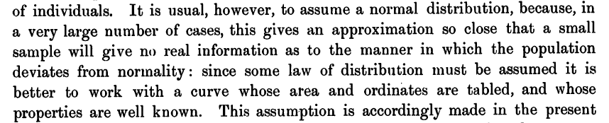
In the era of computational statistics, this advantage matters less, and can sometimes be counterproductive in shifting attention away from the data. 

Data, in fact, are normally-distributed to a lesser degree than a casual observer might think.  Julian Simon, a pioneer in resampling methods (which liberate analysts from normality assumptions), used to teach the normal distribution via heights.  He would draw a bell shaped curve, saying initially that it represented heights.  Then he would amend it by adding a second peak, to distinguish women and men.  Then he would add a long tail to the left: children. Finally, he would produce additional modified curves to represent different regions and ethnic groups. The distribution was normal only after all these groups were filtered out.

Often, data that we think of as normally-distributed, particularly in the social sciences, are that way only after a lot of adjustment.  For example, people often think that intelligence, as represented in IQ scores, is normally-distributed. In fact, IQ tests are engineered to produce scores that are normally distributed.  If the tests produce too many scores at the “intelligent” end of the scale, test engineers add harder questions and drop easy ones. If the tests skew in the opposite direction (too “unintelligent”), the engineers add more easy questions and drop some hard ones.  The fine tuning proceeds until a nicely-shaped normal curve results.   

The term “normal,” by the way, was originally applied in its geometric sense (perpendicular or orthogonal).  Carl Friedrich Gauss applied the term to the familiar bell-shaped distribution because the equations that lay behind it were, at the time, termed orthogonal or normal.  It meant nothing about the typical or usual state of data.