By John Elder, Founder and Chair of Elder Research, Inc.
Last week, in Recidivism, and the Failure of AUC, we saw how the use of “Area Under the Curve” (AUC) concealed bias against African-Americans defendants in a model predicting recidivism, that is, which defendants would re-offend. There, a model varied greatly in its performance characteristics depending on whether the defendant was white or black. Though both situations resulted in virtually identical AUC measures, they led to very different false alarm vs. false dismissal rates. So, AUC failed the analysts relying on it, as it quantified the wrong property of the models and thus missed their vital real-world implications.
In the example last week AUC’s problem was explained as being akin to treating all errors alike. Actually, AUC’s fatal flaw is deeper than that, to the point that the metric should, in fact, never be used! Though it may be intuitively appealing AUC actually is mathematically incoherent in its error treatment, as shown by David Hand in a 2009 KDD keynote talk.
To understand the flaw of AUC and what should replace it we’ll go through the whole process in a brief example. First, note that the curve under which one calculates the area (e.g., ROC or “receiver operating characteristic” curve) illustrates the performance tradeoffs (e.g., sensitivity vs. specificity) of a single classification model as one varies its decision threshold. The threshold is the model output level at which a record is predicted to be a 0 or 1. Thus every different model threshold is a different point on the ROC curve, and the model at that point has its own confusion matrix (or contingency table) of results, summarizing predicted vs. actual 0s vs. 1s.
ROC Curve and Lift Curve
There are actually two kinds of curves analysts use to assess classifier performance and they seem different in their descriptions but are very similar in appearance and utility. The version mentioned already (and last week) is the ROC curve which is a plot of two rates – originally, true positive rate vs. false positive rate, but sometimes sensitivity vs. specificity, or recall vs. precision, etc. The second, which I use most often, is called a Lift Chart or more accurately but less artfully, a Cumulative Response Chart. It plots two proportions: The Y-axis is the proportion of result obtained (such as sales made or fraud found) and the X-axis is proportion of the population treated so far. Importantly, the data is first sorted by model score, so the highest-scoring (most interesting) record is leftmost on the X-axis (is 0) and the lowest (least interesting) record is rightmost on the X-axis (is 1).
Figure 1 is the Lift (Cumulative Response) chart for a model built to predict which home equity loans which will go bad (default). The data had been concentrated (winnowed of many fine loans) to bring the level of defaults up to 20% to make modeling easier for some methods which have a hard time with imbalances in class probabilities. The dark black line is the Lift curve depicting the performance of the model, the blue dashed line shows how the perfect model would perform, and the dotted black line is the expected performance of a random model, which should find 50% of the fraud, for example, after auditing a random 50% of the records. The model in Figure 1 is a classification model, trained on a binary target variable labeled either 0 (for a good loan) or 1 (for bad). “Regression” is in the title as the type of the model was ordinary linear regression.
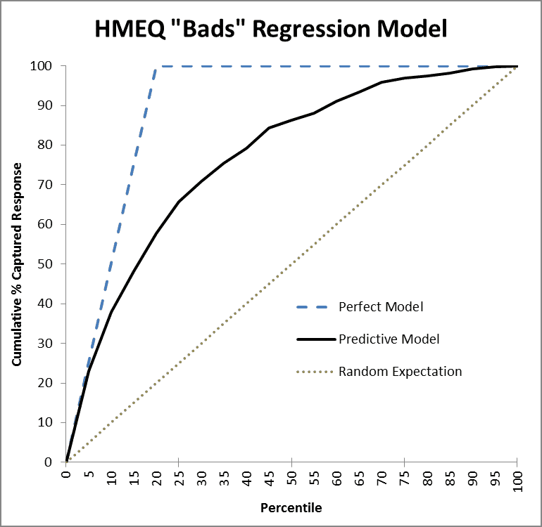
Figure 1: Lift Chart of HMEQ (home equity loans) Model
As an aside, notice that for Lift charts the perfect model doesn’t go straight up; in Figure 1’s example, it takes at least 20% of the cases to get all the bad ones. Unlike the ROC chart, where the perfect model’s AUC can reach 1.0, a Lift chart’s AUC can never reach 1.0; in fact, the maximum possible AUC of a Lift chart will vary according to the problem. (This minor flaw of the AUC metric though is trivial compared to its fatal flaw.)
In Figure 1, the model performs perfectly at first, for high thresholds, and tracks the blue dashed line. But then, as it goes deeper in the list, past the top ~5% of records, it starts to make mistakes and falls off in performance. Still, it does much better than a random ordering of records (the dotted line), by any measure. One could see why AUC might appeal as a way to reduce this curve to a single number. But let’s be smarter than that.
Another different model would create a second solid line. If that line were completely below the existing black line we could confidently throw away the second model for being dominated by the first in every way. But what if it crossed over and was, say, lower earlier but higher in the middle region? We could compare area, yes, but for what reason? Since each point on the curve corresponds to a different error tradeoff, it actually matters more where a line dominates.
Each Point on a Lift Curve corresponds to a Confusion Matrix
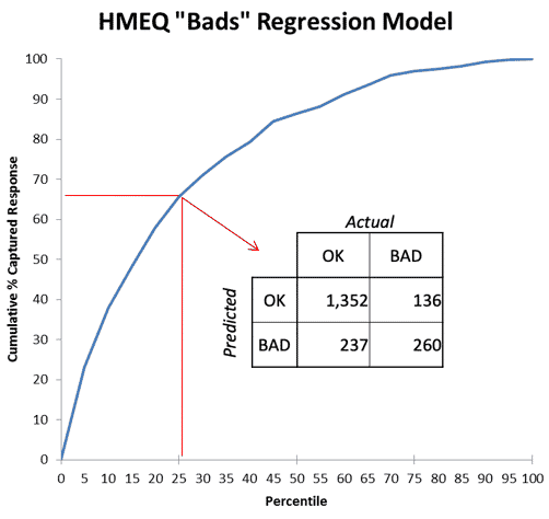
Figure 2: Each point on a Classifier Performance curve corresponds to a Confusion Matrix
Figure 2 highlights a single point on the curve of Figure 1, 25% deep in the list sorted by the model. At that cutoff threshold[1], the classifier has found 260/396 or 66% of the “bads” (defaulters), which proportion is plotted on the Y-axis. Selecting randomly, we would have found only 25% of the “bads.” The model’s “Lift” at that point is thus 66%/25% = 2.64, so it is doing 2.64 times better than the random model. At a higher threshold where the model was still perfect, at X=5%, we can see its lift would be ~4.0. The lift ratio naturally diminishes from there to 1.0 at the end as we go deeper in the list and move up the curve.
[1] I did not record it but it would be lower than the 0.75 one might expect since only 20% of the training data was 1 and modeling shrinks estimates toward the mean. Assume for discussion it was 0.58
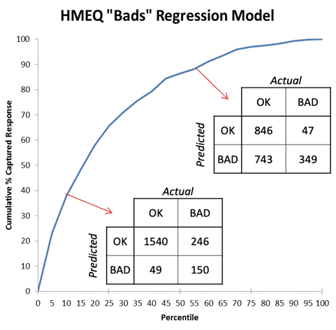
Figure 3: Two points (thresholds for the model) with their corresponding Confusion Matrices
Figure 3 compares two points on the chart (two thresholds for the model) and shows how different their two resulting confusion matrices (contingency charts) are. A model that “cherry picks” cases it calls bad – that is, uses a high threshold — will be a point on the curve near the lower left of the chart, so will be low in both true positive rate and false positive rate. It will have errors of high false dismissal but low false alarm. (In Figure 3, the model 10% deep in the list is right 3/4 of the time when predicting “bad” (150/(150+49)) but misses 5/8 of the bad cases (246/(246+150)).) It is best to choose a high threshold for your model if your problem is one where the cost of a false alarm is much higher than a false dismissal. An example would be an internet search where it’s very important for the top results to be “on topic” and it’s fine to fetch only a fraction of such results.
A low threshold for the decision boundary would place the model on the other end of the curve near the upper right corner, where its errors would reflect rates of low false dismissals but high false alarms. (In Figure 3, the model that calls most cases “bad” finds 7/8 of the bad cases (349/(349+47)) but is wrong 2/3 of the time when it calls one bad (743/(743+349)).) It is best to choose a low threshold for your model if your problem is one where a false alarm’s cost pales in comparison to that of a false dismissal, such as a warning system for an earthquake or tsunami. (As long as the false alarms are not so numerous as the system is completely ignored!)
A real problem will occupy a very narrow part of the ROC or Lift chart space, once it is even partially understood. For instance, in credit scoring, it takes the profit from 5-7 good customers to cover the losses a bank will incur from one defaulting customer. So, it is appropriate to tune a decision system, when predicting credit risk, to have a threshold in a range reflecting that tradeoff. The bank would be very unwise to use a criterion, like AUC, which instead combines information from all over the ROC curve – even parts where a defaulting customer is less important than a normal customer! – to make its decision.
In short, AUC should never be used. It is never the best criterion. It may be “correlated with goodness” in that it rewards good qualities of an ROC curve. But it is always better to examine the problem you are working on to understand its actual relative costs (false alarms vs. false dismissals) or benefits (true positives vs. true negatives) to tune a criterion that makes clear business sense. That will lead to a better solution that more directly meets your goal of minimizing costs or maximizing benefits.
Gains Chart
I recommend using a Gains chart, as depicted in Figure 4. There, the model of Figure 1 has been translated into the language of management ($) for the Y-axis. The output — sales or defaults caught — has been turned into dollars earned or recovered. Also, costs are depicted (the red line); with a fixed cost occurring immediately (setup cost) and a variable cost depending on how deep one goes into the list (“per record” cost). In this example (with high incremental costs), the optimal profit is obtained by investigating only the top 30% of cases as scored by the model.
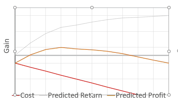
Figure 4: Gains Chart: Positive (blue), Negative (red), Net Gain (orange) vs. depth of list
Lastly, a Note about Constraints
The discussion so far has assumed that you can operate anywhere on the curve. With a marketing application, for example, that is possible; it is just a matter of cost. But with a fraud investigation, on the other hand, each case requires hard work from expert investigators so is also constrained by time and the availability of trained staff. You may only be able to go so deep in the list, no matter how promising the expected payoff. Still, this type of analysis can show what is possible if more resources can be made available – say, new staff hired, or existing staff reassigned and trained. That utility for planning, along with its clarity (and again, speaking the language of management) is why this type of analysis is enthusiastically adopted by leaders and analysts once it is understood.
If the challenge you are dealing with is constrained in its solution approach then you have yet another reason to ignore AUC and do better: compare the performance of models only in the operating region in which you are going to use them.